Network Perturbations: Leave-One-Out and Sequential Node Removal

Companion to networks_random.ipynb. Three graphs with the same size and (nearly) the same mean degree are perturbed by deleting nodes, and the response of global quantities is measured.

Leave-one-out (LOO): delete each node once, recompute, record the change Δ.
Sequential removal: keep deleting nodes, either at random (failure) or hubs first (attack).

import networkx as nx
import numpy as np
import pandas as pd
import matplotlib.pyplot as plt
from matplotlib.colors import Normalize

plt.rcParams.update({
    'axes.spines.top': False, 'axes.spines.right': False,
    'axes.grid': True, 'grid.alpha': 0.25, 'lines.linewidth': 2,
})

The graphs

Density is matched: the ER edge probability is set to \(p = \langle k \rangle / (N-1)\), so that topology rather than edge count drives any difference. (With the original \(p = 0.5\) the ER graph has more than twice the edges of the WS graph.) A Barabási–Albert graph is added as a third case because its heavy-tailed degree distribution makes the attack/failure contrast obvious. All generators are seeded for reproducibility.

N = 30
k = 6                    # target mean degree
p = k / (N - 1)          # ER edge probability matched to WS density  (try 0.5 to compare)
beta = 0.3               # WS rewiring probability
seed = 1234

graphs = {
    'ER': nx.erdos_renyi_graph(N, p, seed=seed),
    'WS': nx.watts_strogatz_graph(N, k, beta, seed=seed),
    'BA': nx.barabasi_albert_graph(N, k // 2, seed=seed),
}

layouts = {
    'ER': nx.spring_layout(graphs['ER'], seed=seed),
    'WS': nx.circular_layout(graphs['WS']),
    'BA': nx.spring_layout(graphs['BA'], seed=seed),
}

Global quantities

average_shortest_path_length fails as soon as the graph is disconnected, so global efficiency \(E = \frac{1}{N(N-1)}\sum_{i\neq j} 1/d_{ij}\) is added: it behaves like an inverse path length but stays defined (unreachable pairs contribute 0). The fraction of nodes in the largest connected component is also tracked.

def global_quantities(G):
    n = G.number_of_nodes()
    connected = n > 1 and nx.is_connected(G)
    giant = max((len(c) for c in nx.connected_components(G)), default=0)
    return {
        'mean degree': 2 * G.number_of_edges() / n if n else np.nan,
        'density': nx.density(G),
        'mean path length': nx.average_shortest_path_length(G) if connected else np.nan,
        'global efficiency': nx.global_efficiency(G),
        'giant component': giant / n if n else 0.0,
    }

baseline = pd.DataFrame({name: global_quantities(G) for name, G in graphs.items()}).T
baseline.round(3)

	mean degree	density	mean path length	global efficiency	giant component
ER	5.6	0.193	2.117	0.547	1.0
WS	6.0	0.207	2.067	0.558	1.0
BA	5.4	0.186	2.018	0.559	1.0

1. Leave-one-out

For every node \(v\): remove it, recompute, store \(\Delta Q_v = Q(G \setminus v) - Q(G)\).

def leave_one_out(G):
    base = global_quantities(G)
    btw = nx.betweenness_centrality(G)
    rows = []
    for v in G.nodes:
        H = G.copy()
        H.remove_node(v)
        q = global_quantities(H)
        rows.append({'node': v, 'degree': G.degree(v), 'betweenness': btw[v],
                     **{f'Δ {key}': q[key] - base[key] for key in base}})
    return pd.DataFrame(rows).set_index('node')

loo = {name: leave_one_out(G) for name, G in graphs.items()}

# the five most damaging single deletions in the WS graph
loo['WS'].sort_values('Δ global efficiency').head().round(4)

	degree	betweenness	Δ mean degree	Δ density	Δ mean path length	Δ global efficiency	Δ giant component
node
29	10	0.1168	-0.4828	-0.0099	0.0663	-0.0141	0.0
20	7	0.0678	-0.2759	-0.0025	0.0417	-0.0078	0.0
26	7	0.0657	-0.2759	-0.0025	0.0417	-0.0076	0.0
24	7	0.0605	-0.2759	-0.0025	0.0294	-0.0057	0.0
5	7	0.0590	-0.2759	-0.0025	0.0294	-0.0057	0.0

How large are the effects, and what predicts them?

summary = {}
for name, df in loo.items():
    b = baseline.loc[name]
    summary[name] = {
        'max |Δ MPL| (%)':            100 * df['Δ mean path length'].abs().max() / b['mean path length'],
        'max |Δ efficiency| (%)':     100 * df['Δ global efficiency'].abs().max() / b['global efficiency'],
        'corr(Δ density, degree)':    df['Δ density'].corr(df['degree']),
        'corr(Δ MPL, betweenness)':   df['Δ mean path length'].corr(df['betweenness']),
        'corr(Δ eff., betweenness)':  df['Δ global efficiency'].corr(df['betweenness']),
    }
pd.DataFrame(summary).T.round(3)

	max \|Δ MPL\| (%)	max \|Δ efficiency\| (%)	corr(Δ density, degree)	corr(Δ MPL, betweenness)	corr(Δ eff., betweenness)
ER	4.118	2.666	-1.0	0.934	-0.927
WS	3.210	2.531	-1.0	0.948	-0.956
BA	10.560	7.985	-1.0	0.981	-0.980

rows = [('degree', 'Δ density'),
        ('betweenness', 'Δ mean path length'),
        ('betweenness', 'Δ global efficiency')]

fig, axes = plt.subplots(len(rows), len(graphs), figsize=(12, 9), sharey='row', sharex='row')
for j, (name, df) in enumerate(loo.items()):
    for i, (x, y) in enumerate(rows):
        ax = axes[i, j]
        ax.axhline(0, color='0.6', lw=1)
        ax.scatter(df[x], df[y], s=40, color='#2a78d6', edgecolor='white', linewidth=1)
        if i == 0:
            ax.set_title(name)
        if j == 0:
            ax.set_ylabel(y)
        ax.set_xlabel(x)
fig.suptitle('Leave-one-out: change in global quantity vs. centrality of the removed node', y=1.0)
fig.tight_layout()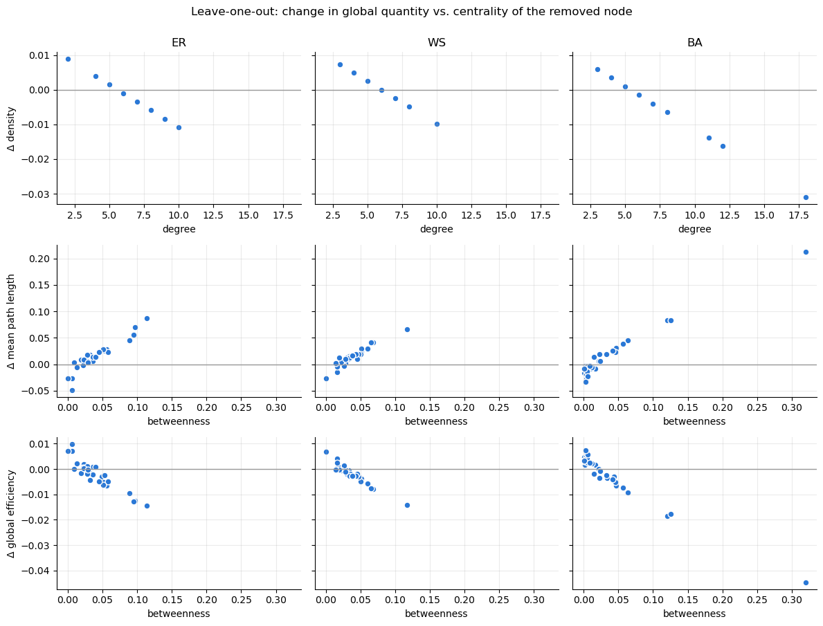

Reading the plots

Row 1 – density (and mean degree) is trivial. Removing a node of degree \(k_v\) gives exactly \(\rho' = 2(M - k_v)/\big((N-1)(N-2)\big)\), a straight line in \(k_v\) (correlation −1). LOO on these quantities only re-ranks nodes by degree. Note also \(\langle k \rangle = \rho\,(N-1)\), so they are the same measurement.
Rows 2–3 – path-based quantities carry information. The impact tracks betweenness, i.e. how many shortest paths run through the node. Effects are small (a few percent) in these dense-ish graphs.
Negative ΔMPL / positive ΔE occur when a peripheral node is removed: its long paths leave the average. That is a normalisation effect, not an improvement of the network – worth pointing out to students.

Impact map

Node colour = Δ global efficiency when that node is removed (red = loss), node size = degree.

vabs = max(df['Δ global efficiency'].abs().max() for df in loo.values())
norm = Normalize(-vabs, vabs)
cmap = plt.cm.RdBu

fig, axes = plt.subplots(1, len(graphs), figsize=(15, 5))
for ax, (name, G) in zip(axes, graphs.items()):
    df = loo[name]
    nx.draw_networkx_edges(G, layouts[name], ax=ax, edge_color='0.75', width=0.8)
    nx.draw_networkx_nodes(G, layouts[name], ax=ax,
                           node_color=[cmap(norm(df.loc[v, 'Δ global efficiency'])) for v in G],
                           node_size=[40 + 25 * G.degree(v) for v in G],
                           edgecolors='white', linewidths=2)
    ax.set_title(name)
    ax.axis('off')
fig.colorbar(plt.cm.ScalarMappable(norm=norm, cmap=cmap), ax=axes, shrink=0.8,
             label='Δ global efficiency after removal');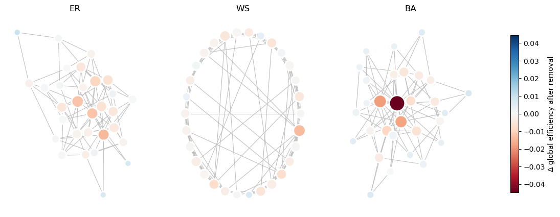

2. Sequential removal: failure vs. attack

Single deletions barely move these graphs. Removing nodes one after another separates them clearly.

random – failure; averaged over many runs (band = 5–95 % range)
degree – attack on the current highest-degree node (recomputed after each removal)
betweenness – attack on the current highest-betweenness node

Tracked: size of the largest component and global efficiency, both relative to the intact graph. Efficiency is averaged over the original \(N(N-1)\) node pairs (removed nodes count as unreachable); otherwise a small surviving fragment such as a single edge would have efficiency 1 and the curve would rise again.

def removal_curve(G, strategy, rng=None):
    H = G.copy()
    N0, E0 = G.number_of_nodes(), nx.global_efficiency(G)
    giant, eff = [1.0], [1.0]
    for _ in range(N0 - 1):
        if strategy == 'random':
            v = rng.choice(list(H.nodes))
        elif strategy == 'degree':
            v = max(H.degree, key=lambda x: x[1])[0]
        elif strategy == 'betweenness':
            b = nx.betweenness_centrality(H)
            v = max(b, key=b.get)
        H.remove_node(v)
        giant.append(max(len(c) for c in nx.connected_components(H)) / N0)
        n = H.number_of_nodes()
        # efficiency counted over the ORIGINAL N(N-1) pairs, so it can only decrease
        eff.append(nx.global_efficiency(H) * n * (n - 1) / (N0 * (N0 - 1)) / E0)
    return np.array(giant), np.array(eff)

n_random = 100
rng = np.random.default_rng(seed)
curves = {}
for name, G in graphs.items():
    rand = np.array([removal_curve(G, 'random', rng) for _ in range(n_random)])  # (runs, 2, N)
    curves[name] = {
        'random': rand,
        'degree': removal_curve(G, 'degree'),
        'betweenness': removal_curve(G, 'betweenness'),
    }

strategy_colors = {'random': '#2a78d6', 'degree': '#eb6834', 'betweenness': '#1baf7a'}
f = np.arange(N) / N          # fraction of nodes removed

fig, axes = plt.subplots(2, len(graphs), figsize=(13, 7), sharex=True, sharey='row')
for j, name in enumerate(graphs):
    for i, label in enumerate(['largest component (fraction of N)', 'global efficiency (relative)']):
        ax = axes[i, j]
        rand = curves[name]['random'][:, i, :]
        ax.fill_between(f, np.percentile(rand, 5, axis=0), np.percentile(rand, 95, axis=0),
                        color=strategy_colors['random'], alpha=0.2, lw=0)
        ax.plot(f, rand.mean(axis=0), color=strategy_colors['random'], label='random (mean)')
        for s in ['degree', 'betweenness']:
            ax.plot(f, curves[name][s][i], color=strategy_colors[s], label=f'{s} attack')
        ax.set_ylim(0, 1.05)
        if i == 0:
            ax.set_title(name)
        else:
            ax.set_xlabel('fraction of nodes removed')
        if j == 0:
            ax.set_ylabel(label)
axes[0, 0].legend(frameon=False)
fig.tight_layout()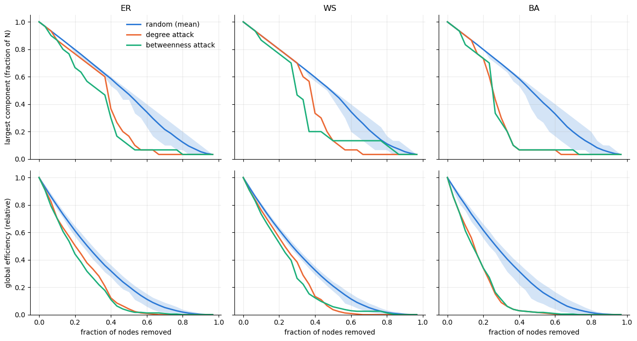

One number per graph: robustness \(R\)

To get back to a single global number per graph, integrate the largest-component curve: \(R = \frac{1}{N}\sum_{q} s(q)\) (Schneider et al., PNAS 2011). \(R \approx 0.5\) is maximally robust, small \(R\) means the network falls apart quickly. The same can be done for the efficiency curve.

R = {}
for name, c in curves.items():
    R[name] = {
        'R random (giant)':       c['random'][:, 0, :].mean(),
        'R degree attack':        c['degree'][0].mean(),
        'R betweenness attack':   c['betweenness'][0].mean(),
        'R_E random (eff.)':      c['random'][:, 1, :].mean(),
        'R_E degree attack':      c['degree'][1].mean(),
    }
pd.DataFrame(R).T.round(3)

	R random (giant)	R degree attack	R betweenness attack	R_E random (eff.)	R_E degree attack
ER	0.485	0.371	0.337	0.322	0.238
WS	0.488	0.376	0.359	0.325	0.254
BA	0.478	0.288	0.286	0.320	0.176

Things to try

Set p = 0.5 (the original ER graph): LOO effects shrink to ~1 % – dense graphs are robust to single deletions.
Vary beta from 0 (ring lattice, all nodes equivalent → all LOO values identical) to 1 (random).
Increase N to 200+: the attack/failure gap in the BA graph widens (use fewer random runs; betweenness attack gets slow).
Edge perturbations: the edge analogue of LOO is removing each edge in turn; its impact tracks nx.edge_betweenness_centrality.